论文 - YOLO v3

YOLO的作者又放出了V3版本，在之前的版本上做出了一些改进，达到了更好的性能。这篇博客介绍这篇论文：YOLOv3: An Incremental Improvement。下面这张图是YOLO V3与RetinaNet的比较。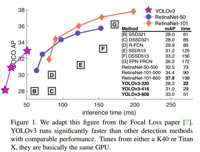

可以使用搜索功能，在本博客内搜索YOLO前作的论文阅读和代码。

YOLO v3比你们不知道高到哪里去了

YOLO v3在保持其一贯的检测速度快的特点前提下，性能又有了提升：输入图像为$320\times 320$大小的图像，可以在$22$ms跑完，mAP达到了$28.2$，这个数据和SSD相同，但是快了$3$倍。在TitanX上，YOLO v3可以在$51$ms内完成，$AP_{50}$的值为$57.9$。而RetinaNet需要$198$ms，$AP_{50}$近似却略低，为$57.5$。

ps：啥是AP

AP就是average precision啦。在detection中，我们认为当预测的bounding box和ground truth的IoU大于某个阈值（如取为$0.5$）时，认为是一个True Positive。如果小于这个阈值，就是一个False Positive。

所谓precision，就是指检测出的框框中有多少是True Positive。另外，还有一个指标叫做recall，是指所有的ground truth里面，有多少被检测出来了。这两个概念都是来自于classification问题，通过设定上面IoU的阈值，就可以迁移到detection中了。

我们可以取不同的阈值，这样就可以绘出一条precisio vs recall的曲线，计算曲线下的面积，就是AP值。COCO中使用了0.5:0.05:0.95十个离散点近似计算（参考COCO的说明文档网页）。detection中常常需要同时检测图像中多个类别的物体，我们将不同类别的AP求平均，就是mAP。

如果我们只看某个固定的阈值，如$0.5$，计算所有类别的平均AP，那么就用$AP_{50}$来表示。所以YOLO v3单拿出来$AP_{50}$说事，是为了证明虽然我的bounding box不如你RetinaNet那么精准（IoU相对较小），但是如果你对框框的位置不是那么敏感（$0.5$的阈值很多时候够用了），那么我是可以做到比你更好更快的。

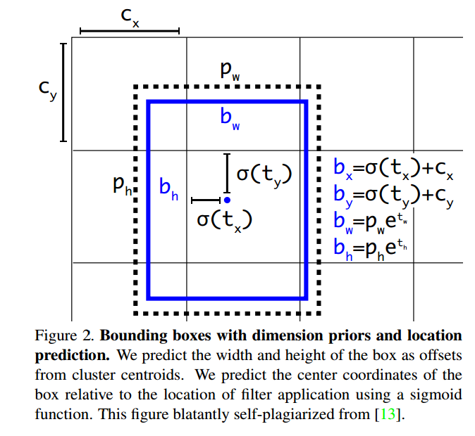
Bounding Box位置的回归

这里和原来v2基本没区别。仍然使用聚类产生anchor box的长宽（下式的$p_w$和$p_h$）。网络预测四个值：$t_x$，$t_y$，$t_w$，$t_h$。我们知道，YOLO网络最后输出是一个$M\times M$的feature map，对应于$M \times M$个cell。如果某个cell距离image的top left corner距离为$(c_x, c_y)$（也就是cell的坐标），那么该cell内的bounding box的位置和形状参数为：

$$\begin{aligned}b_x &= \sigma(t_x) + c_x\\ b_y &= \sigma(t_y) + c_y\\ b_w &= p_w e^{t_w}\\ b_h &= p_h e^{t_h}\end{aligned}$$

PS：这里有一个问题，不管FasterRCNN还是YOLO，都不是直接回归bounding box的长宽（就像这样：$b_w = p_w t_w^\prime$），而是要做一个对数变换，实际预测的是$\log(\cdot)$。这里小小解释一下。

这是因为如果不做变换，直接预测相对形变$t_w^\prime$，那么要求$t_w^\prime > 0$，因为你的框框的长宽不可能是负数。这样，是在做一个有不等式条件约束的优化问题，没法直接用SGD来做。所以先取一个对数变换，将其不等式约束去掉，就可以了。

在训练的时候，使用平方误差损失。

另外，YOLO会对每个bounding box给出是否是object的置信度预测，用来区分objects和背景。这个值使用logistic回归。当某个bounding box与ground truth的IoU大于其他所有bounding box时，target给$1$；如果某个bounding box不是IoU最大的那个，但是IoU也大于了某个阈值（我们取$0.5$），那么我们忽略它（既不惩罚，也不奖励），这个做法是从Faster RCNN借鉴的。我们对每个ground truth只分配一个最好的bounding box与其对应（这与Faster RCNN不同）。如果某个bounding box没有倍assign到任何一个ground truth对应，那么它对边框位置大小的回归和class的预测没有贡献，我们只惩罚它的objectness，即试图减小其confidence。

分类预测

我们不用softmax做分类了，而是使用独立的logisitc做二分类。这种方法的好处是可以处理重叠的多标签问题，如Open Image Dataset。在其中，会出现诸如Woman和Person这样的重叠标签。

FPN加持的多尺度预测

之前YOLO的一个弱点就是缺少多尺度变换，使用FPN中的思路，v3在$3$个不同的尺度上做预测。在COCO上，我们每个尺度都预测$3$个框框，所以一共是$9$个。所以输出的feature map的大小是$N\times N\times [3\times (4+1+80)]$。

然后我们从两层前那里拿feature map，upsample 2x，并与更前面输出的feature map通过element-wide的相加做merge。这样我们能够从后面的层拿到更多的高层语义信息，也能从前面的层拿到细粒度的信息（更大的feature map，更小的感受野）。然后在后面接一些conv做处理，最终得到和上面相似大小的feature map，只不过spatial dimension变成了$2$倍。

照上一段所说方法，再一次在final scale尺度下给出预测。

代码实现

在v3中，作者新建了一个名为yolo的layer，其参数如下：

[yolo]
mask = 0,1,2
## 9组anchor对应9个框框
anchors = 10,13,  16,30,  33,23,  30,61,  62,45,  59,119,  116,90,  156,198,  373,326
classes=20   ## VOC20类
num=9
jitter=.3
ignore_thresh = .5
truth_thresh = 1
random=1

打开yolo_layer.c文件，找到forward部分代码。可以看到，首先，对输入进行activation。注意，如论文所说，对类别进行预测的时候，没有使用v2中的softmax或softmax tree，而是直接使用了logistic变换。

for (b = 0; b < l.batch; ++b){
    for(n = 0; n < l.n; ++n){
        int index = entry_index(l, b, n*l.w*l.h, 0);
        // 对 tx, ty进行logistic变换
        activate_array(l.output + index, 2*l.w*l.h, LOGISTIC);
        index = entry_index(l, b, n*l.w*l.h, 4);
        // 对confidence和C类进行logistic变换
        activate_array(l.output + index, (1+l.classes)*l.w*l.h, LOGISTIC);
    }
}

我们看一下如何计算梯度。

for (j = 0; j < l.h; ++j) {
    for (i = 0; i < l.w; ++i) {
        for (n = 0; n < l.n; ++n) {
            // 对每个预测的bounding box
            // 找到与其IoU最大的ground truth
            int box_index = entry_index(l, b, n*l.w*l.h + j*l.w + i, 0);
            box pred = get_yolo_box(l.output, l.biases, l.mask[n], box_index, i, j, l.w, l.h, net.w, net.h, l.w*l.h);
            float best_iou = 0;
            int best_t = 0;
            for(t = 0; t < l.max_boxes; ++t){
                box truth = float_to_box(net.truth + t*(4 + 1) + b*l.truths, 1);
                if(!truth.x) break;
                float iou = box_iou(pred, truth);
                if (iou > best_iou) {
                    best_iou = iou;
                    best_t = t;
                }
            }
            int obj_index = entry_index(l, b, n*l.w*l.h + j*l.w + i, 4);
            avg_anyobj += l.output[obj_index];
            // 计算梯度
            // 如果大于ignore_thresh, 那么忽略
            // 如果小于ignore_thresh，target = 0
            // diff = -gradient = target - output
            // 为什么是上式，见下面的数学分析
            l.delta[obj_index] = 0 - l.output[obj_index];
            if (best_iou > l.ignore_thresh) {
                l.delta[obj_index] = 0;
            }
            // 这里仍然有疑问，为何使用truth_thresh?这个值是1
            // 按道理，iou无论如何不可能大于1啊。。。
            if (best_iou > l.truth_thresh) {
                // confidence target = 1
                l.delta[obj_index] = 1 - l.output[obj_index];
                int class = net.truth[best_t*(4 + 1) + b*l.truths + 4];
                if (l.map) class = l.map[class];
                int class_index = entry_index(l, b, n*l.w*l.h + j*l.w + i, 4 + 1);
                // 对class进行求导
                delta_yolo_class(l.output, l.delta, class_index, class, l.classes, l.w*l.h, 0);
                box truth = float_to_box(net.truth + best_t*(4 + 1) + b*l.truths, 1);
                // 对box位置参数进行求导
                delta_yolo_box(truth, l.output, l.biases, l.mask[n], box_index, i, j, l.w, l.h, net.w, net.h, l.delta, (2-truth.w*truth.h), l.w*l.h);
            }
        }
    }
}

我们首先来说一下为何confidence（包括后面的classification）的diff计算为何是target - output的形式。对于logistic regression，假设logistic函数的输入是$o = f(x;\theta)$。其中，$\theta$是网络的参数。那么输出$y = h(o)$，其中$h$指logistic激活函数（或sigmoid函数）。那么，我们有：

$$\begin{aligned}P(y=1|x) &= h(o)\\ P(y=0|x) &= 1-h(o)\end{aligned}$$

写出对数极大似然函数，我们有：

$$\log L = \sum y\log h+(1-y)\log(1-h)$$

为了使用SGD，上式两边取相反数，我们有损失函数：

$$J = -\log L = \sum -y\log h-(1-y)\log(1-h)$$

对第$i$个输入$o_i$求导，我们有：

$$\begin{aligned}\frac{\partial J}{\partial o_i} &= \frac{\partial J}{\partial h_i}\frac{\partial h_i}{\partial o_i}\\ &= [-y_i/h_i-(y_i-1)/(1-h_i)] \frac{\partial h_i}{\partial o_i} \\ &= \frac{h_i-y_i}{h_i(1-h_i)} \frac{\partial h_i}{\partial o_i}\end{aligned}$$

根据logistic函数的求导性质，有：

$$\frac{\partial h_i}{\partial o_i} = h_i(1-h_i)$$

所以，有

$$\frac{\partial J}{\partial o_i} = h_i-y_i$$

其中，$h_i$即为logistic激活后的输出，$y_i$为target。由于YOLO代码中均使用diff，也就是-gradient，所以有delta = target - output。

关于logistic回归，还可以参考我的博客：CS229 简单的监督学习方法。

下面，我们看下两个关键的子函数，delta_yolo_class和delta_yolo_box的实现。

// class是类别的ground truth
// classes是类别总数
// index是feature map一维数组里面class prediction的起始索引
void delta_yolo_class(float *output, float *delta, int index, 
  int class, int classes, int stride, float *avg_cat) {
    int n;
    // 这里暂时不懂
    if (delta[index]){
        delta[index + stride*class] = 1 - output[index + stride*class];
        if(avg_cat) *avg_cat += output[index + stride*class];
        return;
    }
    for(n = 0; n < classes; ++n){
        // 见上，diff = target - prediction
        delta[index + stride*n] = ((n == class)?1 : 0) - output[index + stride*n];
        if(n == class && avg_cat) *avg_cat += output[index + stride*n];
    }
}
// box delta这里没什么可说的，就是square error的求导
float delta_yolo_box(box truth, float *x, float *biases, int n, 
  int index, int i, int j, int lw, int lh, int w, int h, 
  float *delta, float scale, int stride) {
    box pred = get_yolo_box(x, biases, n, index, i, j, lw, lh, w, h, stride);
    float iou = box_iou(pred, truth);
    float tx = (truth.x*lw - i);
    float ty = (truth.y*lh - j);
    float tw = log(truth.w*w / biases[2*n]);
    float th = log(truth.h*h / biases[2*n + 1]);

    delta[index + 0*stride] = scale * (tx - x[index + 0*stride]);
    delta[index + 1*stride] = scale * (ty - x[index + 1*stride]);
    delta[index + 2*stride] = scale * (tw - x[index + 2*stride]);
    delta[index + 3*stride] = scale * (th - x[index + 3*stride]);
    return iou;
}

上面，我们遍历了每一个prediction的bounding box，下面我们还要遍历每个ground truth，根据IoU，为其分配一个最佳的匹配。

// 遍历ground truth
for(t = 0; t < l.max_boxes; ++t){
    box truth = float_to_box(net.truth + t*(4 + 1) + b*l.truths, 1);
    if(!truth.x) break;
    // 找到iou最大的那个bounding box
    float best_iou = 0;
    int best_n = 0;
    i = (truth.x * l.w);
    j = (truth.y * l.h);
    box truth_shift = truth;
    truth_shift.x = truth_shift.y = 0;
    for(n = 0; n < l.total; ++n){
        box pred = {0};
        pred.w = l.biases[2*n]/net.w;
        pred.h = l.biases[2*n+1]/net.h;
        float iou = box_iou(pred, truth_shift);
        if (iou > best_iou){
            best_iou = iou;
            best_n = n;
        }
    }
    
    int mask_n = int_index(l.mask, best_n, l.n);
    if(mask_n >= 0){
        int box_index = entry_index(l, b, mask_n*l.w*l.h + j*l.w + i, 0);
        float iou = delta_yolo_box(truth, l.output, l.biases, best_n, 
          box_index, i, j, l.w, l.h, net.w, net.h, l.delta, 
          (2-truth.w*truth.h), l.w*l.h);
        int obj_index = entry_index(l, b, mask_n*l.w*l.h + j*l.w + i, 4);
        avg_obj += l.output[obj_index];
        // 对应objectness target = 1
        l.delta[obj_index] = 1 - l.output[obj_index];
        int class = net.truth[t*(4 + 1) + b*l.truths + 4];
        if (l.map) class = l.map[class];
        int class_index = entry_index(l, b, mask_n*l.w*l.h + j*l.w + i, 4 + 1);
        delta_yolo_class(l.output, l.delta, class_index, class, l.classes, l.w*l.h, &avg_cat);
        ++count;
        ++class_count;
        if(iou > .5) recall += 1;
        if(iou > .75) recall75 += 1;
        avg_iou += iou;
    }
}

Darknet网络架构

引入了ResidualNet的思路（$3\times 3$和$1\times 1$的卷积核，shortcut连接），构建了Darknet-53网络。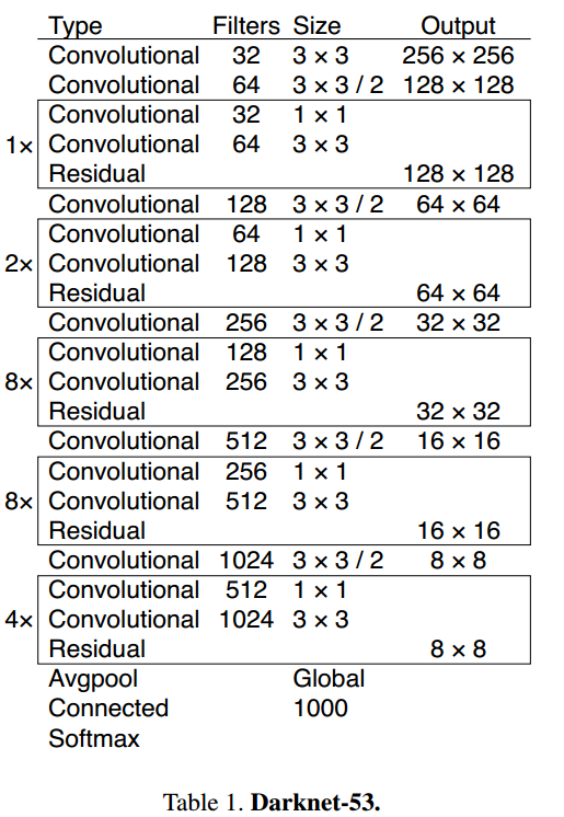

YOLO的优势和劣势

把YOLO v3和其他方法比较，优势在于快快快。当你不太在乎IoU一定要多少多少的时候，YOLO可以做到又快又好。作者还在文章的结尾发起了这样的牢骚：

Russakovsky et al report that that humans have a hard time distinguishing an IOU of .3 from .5! “Training humans to visually inspect a bounding box with IOU of 0.3 and distinguish it from one with IOU 0.5 is surprisingly difficult.” [16] If humans have a hard time telling the difference, how much does it matter?

使用了多尺度预测，v3对于小目标的检测结果明显变好了。不过对于medium和large的目标，表现相对不好。这是需要后续工作进一步挖局的地方。

下面是具体的数据比较。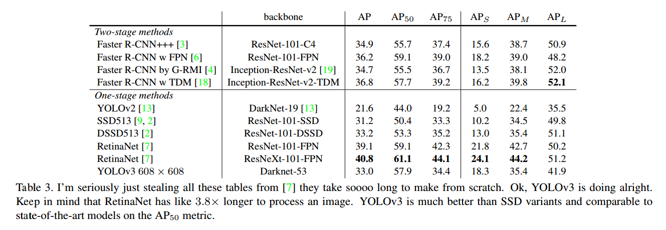

我们是身经百战，见得多了

作者还贴心地给出了什么方法没有奏效。

• anchor box坐标$(x, y)$的预测。预测anchor box的offset，no stable，不好。
• 线性offset预测，而不是logistic。精度下降。
• focal loss。精度下降。
• 双IoU阈值，像Faster RCNN那样。效果不好。

参考资料

下面是一些可供利用的参考资料：

• YOLO的项目主页Darknet YOLO
• 作者主页上的paper链接
• 知乎专栏上的全文翻译
• FPN论文Feature pyramid networks for object detection
• 知乎上的解答：AP是什么，怎么计算