CS131-描述图像的特征(SIFT)

SIFT(尺度不变特征变换，Scale Invariant Feature Transform),最早由Lowe提出，目的是为了解决目标检测（Object Detection）问题中提取图像特征的问题。从名字可以看出，SIFT的优势就在于对尺度变换的不变性，同时SIFT还满足平移变换和旋转变换下的不变性，并对光照变化和3D视角变换有一定的不变性。它的主要步骤如下：

• scale space上的极值检测。使用DoG在不同的scaleast和image position下找到interest point。
• interest point的localization。对上面的interest point进行稳定度检测，并确定其所在的scale和position。
• 确定方向。通过计算图像的梯度图，确定key point的方向，下一步的feature operation就是在这个方向，scale和position上进行的。
• 确定key point的描述子。使用图像的局部梯度作为key point的描述子，最终构成SIFT特征向量。

SIFT介绍

上讲中介绍的Harris角点方法计算简便，并具有平移不变性和旋转不变性。特征$f$对某种变换$\mathcal{T}$具有不变性，是指在经过变换后原特征保持不变，也就是$f(I) = f(\mathcal{T}(I))$。但是Harris角点不具有尺度变换不变性，如下图所示。当图像被放大后，原图的角点被判定为了边缘点。

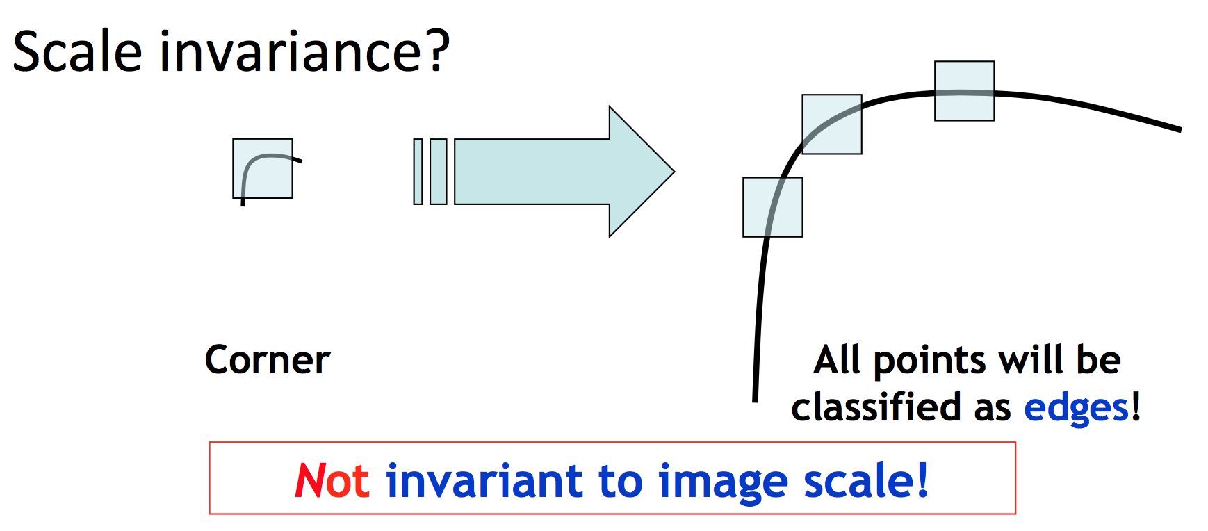
而我们想要得到一种对尺度变换保持不变性的特征计算方法。例如图像patch的像素平均亮度，如下图所示。region size缩小为原始的一半后，亮度直方图的形状不变，即平均亮度不变。

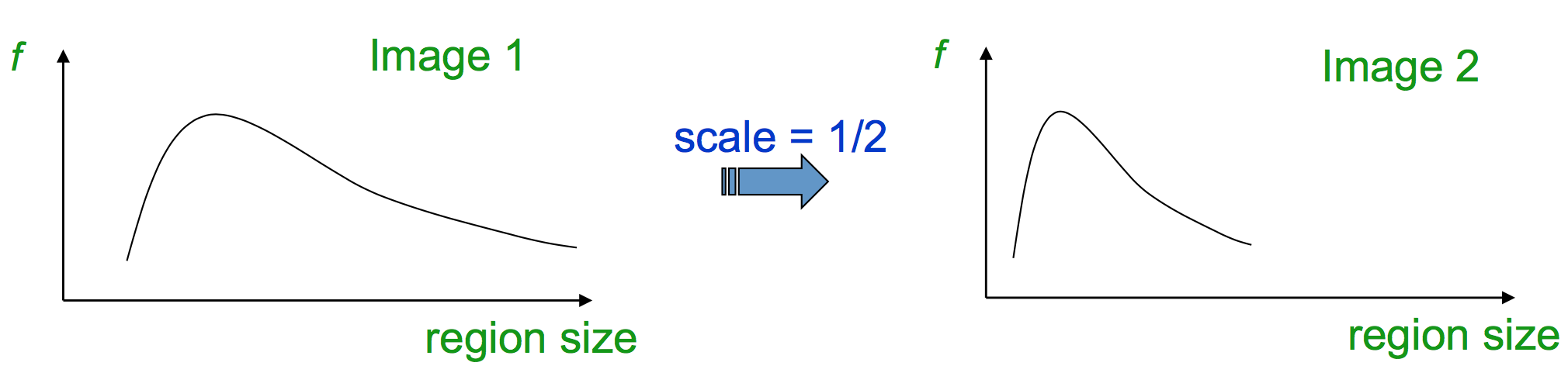
而Lowe想到了使用局部极值来作为feature来保证对scale变换的不变性。在算法的具体实现中，他使用DoG来获得局部极值。

Lowe的论文中也提到了SIFT特征的应用。SIFT特征可以产生稠密（dense）的key point，例如一张500x500像素大小的图像，一般可以产生~2000个稳定的SIFT特征。在进行image matching和recognition时，可以将ref image的SIFT特征提前计算出来保存在数据库中，并计算待处理图像的SIFT特征，根据特征向量的欧氏距离进行匹配。

这篇博客主要是Lowe上述论文的读书笔记，按照SIFT特征的计算步骤进行组织。

尺度空间极值的检测方法

前人研究已经指出，在一系列合理假设下，高斯核是唯一满足尺度不变性的。所谓的尺度空间，就是指原始图像$I(x,y)$和可变尺度的高斯核$G(x,y,\sigma)$的卷积结果。如下式所示：

$$L(x,y,\sigma) = G(x,y,\sigma)\ast I(x,y)$$

其中，$G(x,y, \sigma) = \frac{1}{2\pi\sigma^2}\exp(-(x^2+y^2)/2\sigma^2)$。不同的$\sigma$代表不同的尺度。

DoG(difference of Gaussian)函数定义为不同尺度的高斯核与图像卷积结果之差，即，

$$D(x,y,\sigma) = L(x,y,k\sigma) - L(x,y,\sigma)$$

如下图所示，输入的图像重复地与高斯核进行卷积得到结果图像$L$（左侧），这样构成了一个octave。相邻的$L$之间作差得到DoG图像（右侧）。当一个octave处理完之后，将当前octave的最后一张高斯卷积结果图像降采样两倍，按照前述方法构造下一个octave。在图中，我们将一个octave划分为$s$个间隔（即$s+1$个图像）时，设$\sigma$最终变成了2倍（即$\sigma$加倍）。那么，显然有相邻两层之间的$k = 2^{1/s}$。不过为了保证首尾两张图像也能够计算差值，我们实际上需要再补上两张（做一个padding），也就是说一个octave内的总图像为$s+3$（下图中的$s=2$）。

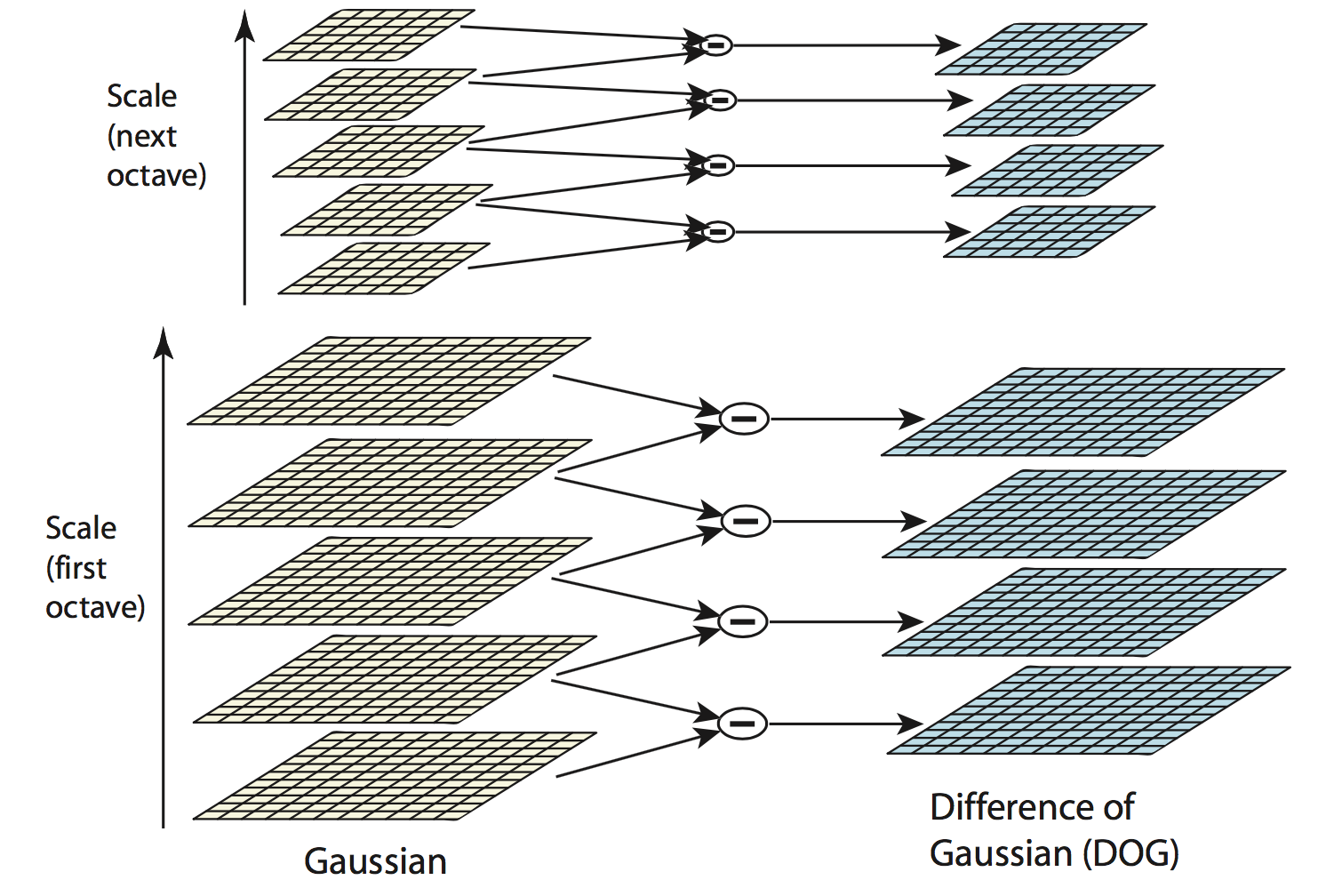
为何我们要费力气得到DoG呢？论文中作者给出的解释是：DoG对scale-normalized后的Guassian Laplace函数$\sigma^2\Delta G$提供了足够的近似。其中前面的$\sigma^2$系数正是为了保证尺度不变性。而前人的研究则指出，$\sigma \Delta G$函数的极值，和其他一大票其他function比较时，能够提供最稳定的feature。

对于高斯核函数，有以下性质：

$$\frac{\partial G}{\partial \sigma} = \sigma \Delta G$$

我们将式子左侧的微分变成差分，得到了下式：

$$\sigma\Delta G \approx \frac{G(x,y,k\sigma)-G(x,y,\sigma)}{k\sigma - \sigma}$$

也就是：

$$G(x,y,k\sigma)-G(x,y,\sigma) \approx (k-1)\sigma^2 \Delta G$$

当$k=1$时，上式的近似误差为0（即上面的$s=\infty$，也就是说octave的划分是连续的）。但是当$k$较大时，如$\sqrt{2}$（这时$s=2$，octave划分十分粗糙了），仍然保证了稳定性。同时，由于相邻两层的比例$k$是定值，所以$k-1$这个因子对于检测极值没有影响。我们在计算时，无需除以$k-1$。

构造完了DoG图像金字塔，下面我们的任务就是检测其中的极值。如下图，对于每个点，我们将它与金字塔中相邻的26个点作比较，找到局部极值。

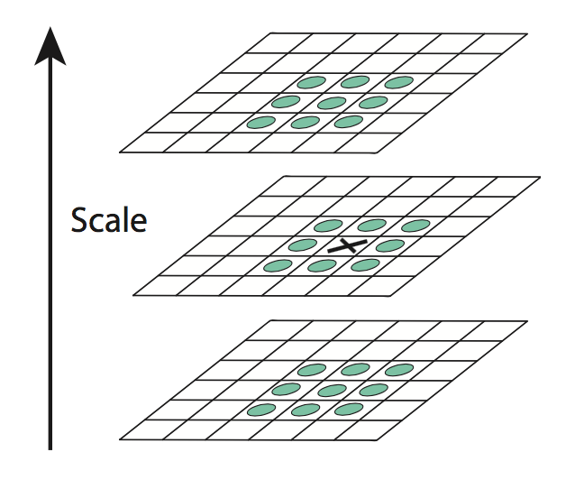
另外，我们将输入图像行列预先使用线性插值的方法resize为原来的2倍，获取更多的key point。

此外，在Lowe的论文中还提到了使用DoG的泰勒展开和海森矩阵进行key point的精细确定方法，并对key point进行过滤。这里也不再赘述了。

128维feature的获取

我们需要在每个key point处提取128维的特征向量。这里结合CS131课程作业2的相关练习作出说明。对于每个key point，我们关注它位于图像金字塔中的具体层数以及像素点位置，也就是说通过索引pyramid{scale}(y, x)就可以获取key point。我们遍历key point，为它们赋予一个128维的特征向量。

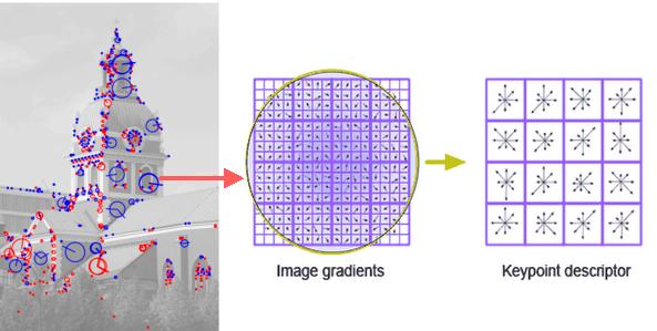
我们选取point周围16x16大小的区域，称为一个patch。将其分为4x4共计16个cell。这样，每个cell内共有像素点16个。对于每个cell，我们计算它的局部梯度方向直方图，直方图共有8个bin。也就是说每个cell可以得到一个8维的特征向量。将16个cell的特征向量首尾相接，就得到了128维的SIFT特征向量。在下面的代码中，使用变量patch_mag和patch_theta分别代表patch的梯度幅值和角度，它们可以很简单地使用卷积和数学运算得到。

patch_mag = sqrt(patch_dx.^2 + patch_dy.^2);
patch_theta = atan2(patch_dy, patch_dx);  % atan2的返回结果在区间[-pi, pi]上。
patch_theta = mod(patch_theta, 2*pi);   % 这里我们要将其转换为[0, 2pi]

之后，我们需要获取key point的主方向。其定义可见slide，即为key point扩展出来的patch的梯度方向直方图的峰值对应的角度。

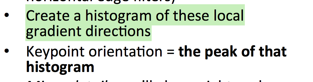
所以我们首先应该设计如何构建局部梯度方向直方图。我们只要将[0, 2pi]区间划分为若干个bin，并将patch内的每个点使用其梯度大小向对应的bin内投票即可。如下所示：

function [histogram, angles] = ComputeGradientHistogram(num_bins, gradient_magnitudes, gradient_angles)
% Compute a gradient histogram using gradient magnitudes and directions.
% Each point is assigned to one of num_bins depending on its gradient
% direction; the gradient magnitude of that point is added to its bin.
%
% INPUT
% num_bins: The number of bins to which points should be assigned.
% gradient_magnitudes, gradient angles:
%       Two arrays of the same shape where gradient_magnitudes(i) and
%       gradient_angles(i) give the magnitude and direction of the gradient
%       for the ith point. gradient_angles ranges from 0 to 2*pi
%                                      
% OUTPUT
% histogram: A 1 x num_bins array containing the gradient histogram. Entry 1 is
%       the sum of entries in gradient_magnitudes whose corresponding
%       gradient_angles lie between 0 and angle_step. Similarly, entry 2 is for
%       angles between angle_step and 2*angle_step. Angle_step is calculated as
%       2*pi/num_bins.

% angles: A 1 x num_bins array which holds the histogram bin lower bounds.
%       In other words, histogram(i) contains the sum of the
%       gradient magnitudes of all points whose gradient directions fall
%       in the range [angles(i), angles(i + 1))

    angle_step = 2 * pi / num_bins;
    angles = 0 : angle_step : (2*pi-angle_step);

    histogram = zeros(1, num_bins);
    num = numel(gradient_angles);
    for n = 1:num
        index = floor(gradient_angles(n) / angle_step) + 1;
        histogram(index) = histogram(index) + gradient_magnitudes(n);
    end    
end

Lowe论文中推荐的bin数目为36个，计算主方向的函数如下：

function direction = ComputeDominantDirection(gradient_magnitudes, gradient_angles)
% Computes the dominant gradient direction for the region around a keypoint
% given the scale of the keypoint and the gradient magnitudes and gradient
% angles of the pixels in the region surrounding the keypoint.
%
% INPUT
% gradient_magnitudes, gradient_angles:
%   Two arrays of the same shape where gradient_magnitudes(i) and
%   gradient_angles(i) give the magnitude and direction of the gradient for
%   the ith point.

    % Compute a gradient histogram using the weighted gradient magnitudes.
    % In David Lowe's paper he suggests using 36 bins for this histogram.
    num_bins = 36;
    % Step 1:
    % compute the 36-bin histogram of angles using ComputeGradientHistogram()
    [histogram, angle_bound] = ComputeGradientHistogram(num_bins, gradient_magnitudes, gradient_angles);
    % Step 2:
    % Find the maximum value of the gradient histogram, and set "direction"
    % to the angle corresponding to the maximum. (To match our solutions,
    % just use the lower-bound angle of the max histogram bin. (E.g. return
    % 0 radians if it's bin 1.)
    [~, max_index] = max(histogram);
    direction = angle_bound(max_index);
end

之后，我们更新patch内各点的梯度方向，计算其与主方向的夹角，作为新的方向。并将梯度进行高斯平滑。

patch_theta = patch_theta - ComputeDominantDirection(patch_mag, patch_theta);;
patch_theta = mod(patch_theta, 2*pi);
patch_mag = patch_mag .* fspecial('gaussian', patch_size, patch_size / 2); % patch_size = 16

遍历cell，计算feature如下：

feature = [];
row_iter = 1;
for y = 1:num_histograms
    col_iter = 1;
    for x = 1:num_histograms
        cell_mag = patch_mag(row_iter: row_iter + pixelsPerHistogram - 1, ...
                             col_iter: col_iter + pixelsPerHistogram - 1);
        cell_theta = patch_theta(row_iter: row_iter + pixelsPerHistogram - 1, ...
                             col_iter: col_iter + pixelsPerHistogram - 1);
        [histogram, ~] = ComputeGradientHistogram(num_angles, cell_mag, cell_theta);
        feature = [feature, histogram];
        col_iter = col_iter + pixelsPerHistogram;
    end
    row_iter = row_iter + pixelsPerHistogram;
end

最后，对feature做normalization。首先将feature化为单位长度，并将其中太大的分量进行限幅（如0.2的阈值），之后再重新将其转换为单位长度。

这样，就完成了SIFT特征的计算。在Lowe的论文中，有更多对实现细节的讨论，这里只是跟随课程slide和作业走完了算法流程，不再赘述。

应用：图像特征点匹配

和Harris角点一样，SIFT特征可以用作两幅图像的特征点匹配，并且具有多种变换不变性的优点。对于两幅图像分别计算得到的特征点SIFT特征向量，可以使用下面简单的方法搜寻匹配点。计算每组点对之间的欧式距离，如果最近的距离比第二近的距离小得多，那么可以认为有一对成功匹配的特征点。其MATLAB代码如下，其中descriptor是两幅图像的SIFT特征向量。阈值默认为取做0.7。

function match = SIFTSimpleMatcher(descriptor1, descriptor2, thresh)
% SIFTSimpleMatcher
%   Match one set of SIFT descriptors (descriptor1) to another set of
%   descriptors (decriptor2). Each descriptor from descriptor1 can at
%   most be matched to one member of descriptor2, but descriptors from
%   descriptor2 can be matched more than once.
%   
%   Matches are determined as follows:
%   For each descriptor vector in descriptor1, find the Euclidean distance
%   between it and each descriptor vector in descriptor2. If the smallest
%   distance is less than thresh*(the next smallest distance), we say that
%   the two vectors are a match, and we add the row [d1 index, d2 index] to
%   the "match" array.
%   
% INPUT:
%   descriptor1: N1 * 128 matrix, each row is a SIFT descriptor.
%   descriptor2: N2 * 128 matrix, each row is a SIFT descriptor.
%   thresh: a given threshold of ratio. Typically 0.7
%
% OUTPUT:
%   Match: N * 2 matrix, each row is a match.
%          For example, Match(k, :) = [i, j] means i-th descriptor in
%          descriptor1 is matched to j-th descriptor in descriptor2.
    if ~exist('thresh', 'var'),
        thresh = 0.7;
    end

    match = [];
    [N1, ~] = size(descriptor1);
    for i = 1:N1
        fea = descriptor1(i, :);
        err = bsxfun(@minus, fea, descriptor2);
        dis = sqrt(sum(err.^2, 2));
        [sorted_dis, ind] = sort(dis, 1);
        if sorted_dis(1) < thresh * sorted_dis(2)
            match = [match; [i, ind(1)]];
        end
    end
end

接下来，我们可以使用最小二乘法计算两幅图像之间的仿射变换矩阵（齐次变换矩阵）$H$。其中$H$满足：

$$Hp_{\text{before}} = p_{\text{after}}$$

其中

$$p = \begin{bmatrix}x \\\\ y \\\\ 1\end{bmatrix}$$

对上式稍作变形，有

$$p_{\text{before}}^\dagger H^\dagger = p_{\text{after}}\dagger$$

就可以使用标准的最小二乘正则方程进行求解了。代码如下：

function H = ComputeAffineMatrix( Pt1, Pt2 )
%ComputeAffineMatrix
%   Computes the transformation matrix that transforms a point from
%   coordinate frame 1 to coordinate frame 2
%Input:
%   Pt1: N * 2 matrix, each row is a point in image 1
%       (N must be at least 3)
%   Pt2: N * 2 matrix, each row is the point in image 2 that
%       matches the same point in image 1 (N should be more than 3)
%Output:
%   H: 3 * 3 affine transformation matrix,
%       such that H*pt1(i,:) = pt2(i,:)

    N = size(Pt1,1);
    if size(Pt1, 1) ~= size(Pt2, 1),
        error('Dimensions unmatched.');
    elseif N<3
        error('At least 3 points are required.');
    end

    % Convert the input points to homogeneous coordintes.
    P1 = [Pt1';ones(1,N)];
    P2 = [Pt2';ones(1,N)];

    H = P1*P1'\P1*P2';
    H = H';

    % Sometimes numerical issues cause least-squares to produce a bottom
    % row which is not exactly [0 0 1], which confuses some of the later
    % code. So we'll ensure the bottom row is exactly [0 0 1].
    H(3,:) = [0 0 1];
end

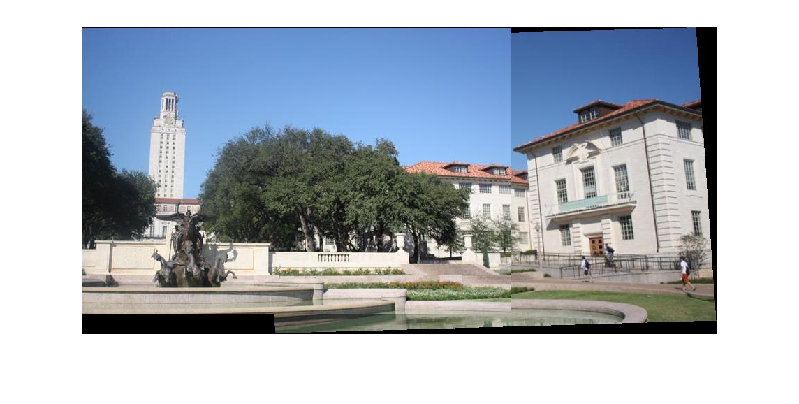
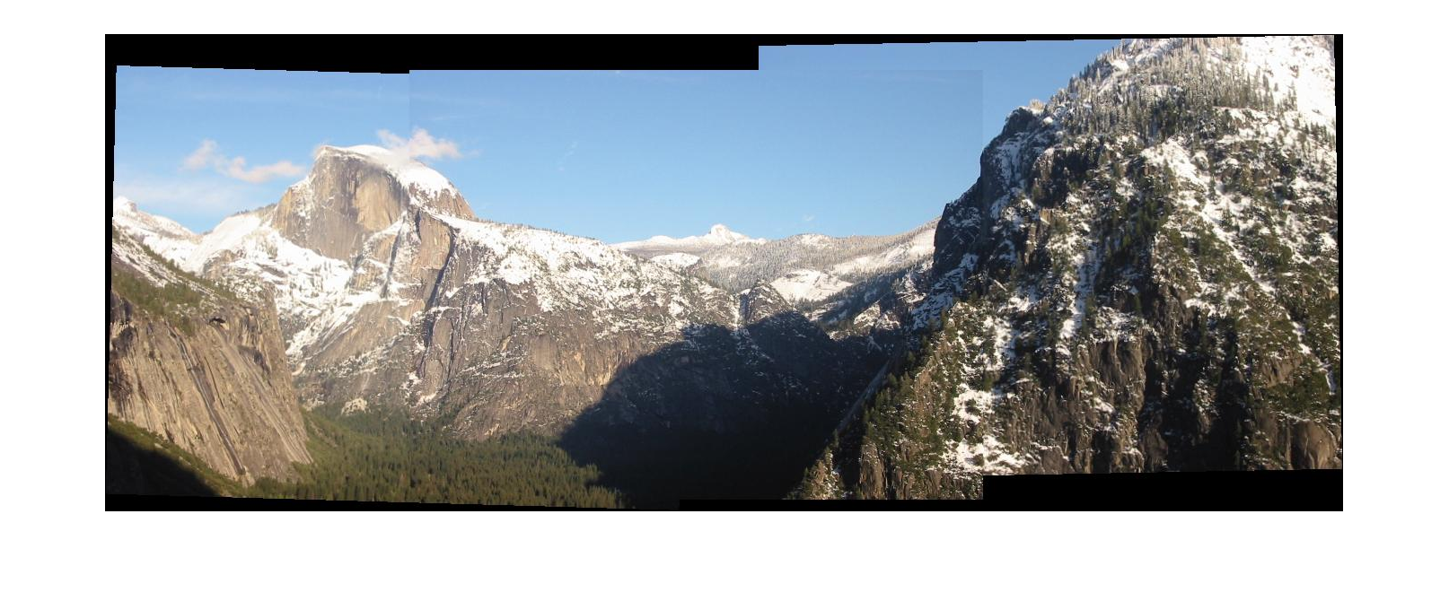
作业中的其他例子也很有趣，这里不再多说了。贴上两张图像拼接的实验结果吧~